这篇博客主要想记录一下学习Ross Girshick大神的py-faster-rcnn源码的笔记,方便以后翻看。
博主项目里只用tensorflow,无奈很多好的模型都用caffe,加上caffe确实比tensorflow好读懂,所以顺带学一遍caffe,顺便学习贾大神写的caffe c++源码。
faster rcnn结构还是比较复杂的,下面开始解读一下源码:
训练过程概况:
由train_faster_rcnn_alt_opt.py可以看到整个训练过程,分为一下几个部分,下面文章会就这几个训练过程讲解代码:
- Stage 1 RPN, init from ImageNet model
- Stage 1 RPN, generate proposals
- Stage 1 Fast R-CNN using RPN proposals, init from ImageNet model
- Stage 2 RPN, init from stage 1 Fast R-CNN model
- Stage 2 RPN, generate proposals
- Stage 2 Fast R-CNN, init from stage 2 RPN R-CNN model
主要是两个循环:训练RPN,用RPN生成的proposal训练Fast R-CNN,再训练RPN,再用RPN生成的proposal训练Fast R-CNN。
我们可以获取所有阶段的pt文件看模型结构,重点看以下几个环节:
RPN train:
 RPN test, proposal生成:
 Fast R-CNN train:
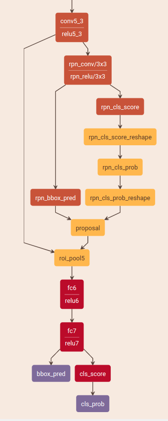
 Fast R-CNN test:
其中包含了几个重要的layer,下面会展开。
RoIDataLayer, AnchorTargetLayer, ProposalLayer, ProposalTargetLayer, ROIPooing, SmoothL1Loss layer
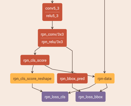
RPN train
- vgg提取特征(最后是conv5_3,relu5_3)
- rpn_conv(3x3卷积,shape=(1,512,h,w))
- 两个1x1卷积:
- rpn_cls_score,shape=(1,18,h,w),可以理解为9个anchor在每个像素(h,w)对应的原图上是否是物体的概率,之后转换成rpn_cls_score_reshape,shape=(1,2,9*h,w)
- rpn_bbox_pred,shape=(1,36,h,w), 可以理解为9个anchor的4个坐标点在每个像素(h,w)对应的原图上的偏差
- AnchorTargetLayer得到每个anchor对应的label,bbox坐标
- 分别计算各自的loss(rpn_loss_cls(SoftmaxWithLoss), rpn_loss_bbox(SmoothL1Loss))
RoIDataLayer:
RoIDataLayer在RPN训练中返回data,im_info,gt_boxes。
- data,含有所有resize后图片array的blob
- im_info=(h, w, scale), scale 是最小边resize到600的需要乘的系数=float(target_size) / float(im_size_min)
- gt_boxes=(x1, y1, x2, y2, label),具体区域的坐标和分类标签
AnchorTargetLayer:
layer {
  name: 'rpn-data'
  type: 'Python'
  bottom: 'rpn_cls_score'
  bottom: 'gt_boxes'
  bottom: 'im_info'
  bottom: 'data'
  top: 'rpn_labels'
  top: 'rpn_bbox_targets'
  top: 'rpn_bbox_inside_weights'
  top: 'rpn_bbox_outside_weights'
  python_param {
    module: 'rpn.anchor_target_layer'
    layer: 'AnchorTargetLayer'
    param_str: "'feat_stride': 16"
  }
}
这一层是针对每个anchor生成target和label用于计算loss。 分类的label为1(物体),0(非物体),-1(忽略)。 如果分类lable>0则进行box regression 这里生成的anchor就是预测的proposal。
首先得到原有图片大小:rpn_cls_score中feature map × feat_stride(16)
接着得到anchor(9个,包含了三种大小,尺寸的组合)对应原图中bbox,一共有14x14x9个
保留那些不超出图片大小的anchor, shape =(N, 4)(n<14x14x9, 下面计算只用这些数量的anchor,但是最后返回包含去掉的anchor)
通过覆盖度阈值(inter_area / anchor_area U gt_area),给所有anchor标签1,0,-1。覆盖度最大的,已经与gt覆盖超过0.7的为1,小于0.3的为0,其余的为-1。
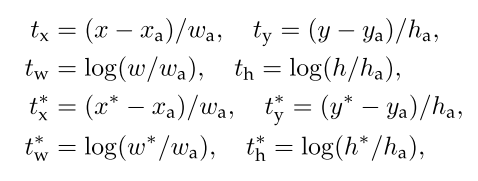
计算bbox_targets, shape=(N, 4), bbox_targets是anchor与gt的偏差, 由下面公式得到, P=anchor, G=gt

bbox_inside_weights, shape=(N, 4), 标记为物体的anchor值为(1,1,1,1),其余为(0,0,0,0),保证在计算smooth l1的时候,我们是对前景做回归,忽略其他。
bbox_outside_weights, shape=(N, 4), 如果TRAIN.RPN_POSITIVE_WEIGHT(p) < 0, 前景和背景的权重都为 1 / num(anchor), 如果0 < TRAIN.RPN_POSITIVE_WEIGHT(p) < 1,前景权重为 p * 1 / {num positives},背景为(1-p)/ {num negetive},其余为(0,0,0,0)。这样做是因为前景和背景的数量差异很大。
bbox_inside_weights 和 bbox_outside_weights详细使用看下面smoothl1loss层解析。
接下来将所有的返回值映射回原有anchor数量的数组,就是加上因为超出图片大小而去掉的anchor,把N转化成原来的14x14x9
labels = _unmap(labels, total_anchors, inds_inside, fill=-1)
bbox_targets = _unmap(bbox_targets, total_anchors, inds_inside, fill=0)
bbox_inside_weights = _unmap(bbox_inside_weights, total_anchors, inds_inside, fill=0)
bbox_outside_weights = _unmap(bbox_outside_weights, total_anchors, inds_inside, fill=0)
这里得到:
- labels (14x14x9, 1)
- bbox_targets (14x14x9, 4)
- bbox_inside_weights (14x14x9, 4)
- bbox_outside_weights (14x14x9, 4)
reshape后,返回四个值为: height=14, width=14, A=9
- labels (1, 1, A * height, width)
- bbox_targets (1, A * 4, height, width)
- bbox_targets指的是anchor与gt的偏差,shape具体是(1, 9 * 4, 14, 14),以前4个channel为例,第一个channel的feature map每一个值是每个位置中心点x方向的补偿值dx,第二个channel的feature map每一个值是每个位置中心点y方向的补偿值dy,第三个channel的feature map每一个值是每个位置宽度的补偿值dw,第四个channel的feature map每一个值是每个位置长度的补偿值dh,接下来的channel都是,每4个属于一个anchor的偏移值。
- bbox_inside_weights (1, A * 4, height, width)
- bbox_outside_weights (1, A * 4, height, width)
SmoothL1Loss layer
layer {
  name: "rpn_loss_bbox"
  type: "SmoothL1Loss"
  bottom: "rpn_bbox_pred"
  bottom: "rpn_bbox_targets"
  bottom: 'rpn_bbox_inside_weights'
  bottom: 'rpn_bbox_outside_weights'
  top: "rpn_loss_bbox"
  loss_weight: 1
  smooth_l1_loss_param { sigma: 3.0 }
}
计算损失函数论文使用:
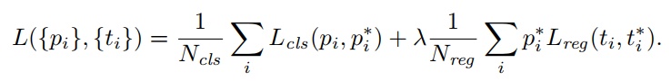
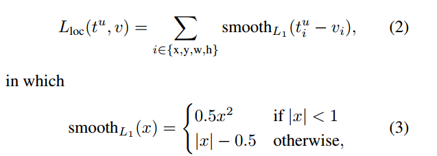
- Lreg(ti, t∗i ) = R(ti − t∗i ), R是smoothl1loss
- rpn_bbox_pred anchor与预测的偏移量 ti
- rpn_bbox_targets anchor与gt的偏差 t*i
实际的SmoothL1Loss计算和文中提到的有出入。
先计算w_in * (ti - ti), 再计算w_out * SmoothL1(w_in * (ti - ti)), 最后相加除以num总数(相当于乘上1/N_reg)。这里的w_in是bbox_inside_weights,w_out是bbox_outside_weights。
所以loss function最后一部分应该是:
\(\lambda1/N_{reg} \Sigma w_{out} L_{reg}(w_{in}(t_i, t_i^*))\)
w_in在这里面的含义是只计算前景的回归,所以他的定义就是除了前景为(1,1,1,1),其余的都是(0,0,0,0),而w_out是为了在函数中加入前景和背景的权重,因为有的时候前景和背景的数量相差悬殊,但是论文中用的是1:1的数量,所以对应代码是w_out = np.ones((1, 4)) * 1.0 / numexamples,相当于前景和背景的w_out都是(1/N_reg,1/N_reg,1/N_reg,1/N_reg)。
虽然这样对应上了源码的实现,但是相当于最后smoothl1乘了1/Nreg^2,不是很理解,而且也不知道怎么解析论文里面的里面写到pi是0,1的细节,我觉得这个作用和w_in效果是一样的,就当是w_in好了。
caffe_gpu_sub(
      count,
      bottom[0]->gpu_data(),   // bbox_pred
      bottom[1]->gpu_data(),   // bbox_targets
      diff_.mutable_gpu_data());    // d := b0 - b1
  if (has_weights_) {
    // apply "inside" weights
    caffe_gpu_mul(
        count,
        bottom[2]->gpu_data(),
        diff_.gpu_data(),
        diff_.mutable_gpu_data());  // d := w_in * (b0 - b1)
  }
  SmoothL1Forward<Dtype><<<CAFFE_GET_BLOCKS(count), CAFFE_CUDA_NUM_THREADS>>>(
      count, diff_.gpu_data(), errors_.mutable_gpu_data(), sigma2_);
  CUDA_POST_KERNEL_CHECK;

  if (has_weights_) {
    // apply "outside" weights
    caffe_gpu_mul(
        count,
        bottom[3]->gpu_data(),
        errors_.gpu_data(),
        errors_.mutable_gpu_data());  // d := w_out * SmoothL1(w_in * (b0 - b1))
  }
  Dtype loss;
  caffe_gpu_dot(count, ones_.gpu_data(), errors_.gpu_data(), &loss);
  top[0]->mutable_cpu_data()[0] = loss / bottom[0]->num();
}
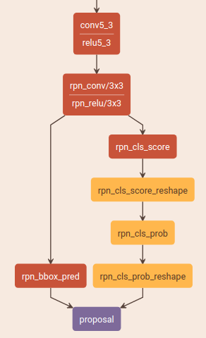
RPN test (generate proposals)
这一层是用来生成fast rcnn所需要的region proposal
- vgg提取特征(最后是conv5_3,relu5_3)
- rpn_conv(3x3卷积,shape=(1,512,h,w))
- 两个1x1卷积:
- rpn_cls_score,shape=(1,18,h,w),可以理解为9个anchor在每个像素(h,w)对应的原图上是否是物体的概率,包涵下面几个操作。
- rpn_cls_score_reshape(shape=(1,2,9xh,w)),这里的reshape是方便后面softmax计算
- rpn_cls_pro = softmax(rpn_cls_score_reshape)
- rpn_cls_pro_reshape(shape=(1,18,h,w)), 前面九个是背景概率,后面就个是前景概率,后面计算会用到的是前景概率
- rpn_bbox_pred,shape=(1,36,h,w), 可以理解为9个anchor的4个坐标点在每个像素(h,w)与proposal预测对应4个坐标点的偏差
- rpn_cls_score,shape=(1,18,h,w),可以理解为9个anchor在每个像素(h,w)对应的原图上是否是物体的概率,包涵下面几个操作。
- ProposalLayer结合上面结果生成原图上预测的object proposals,通过nms得到最后的proposals,scores
ProposalLayer: (整个环节与fast rcnn类似)
将RPN结果(per-anchor scores and bbox regression estimates)转为原图上的object proposals。
layer {
  name: 'proposal'
  type: 'Python'
  bottom: 'rpn_cls_prob_reshape'
  bottom: 'rpn_bbox_pred' # 用于回归预测的proposal bbox
  bottom: 'im_info' # shape = (H, W, scaler) scale:缩放比例
  top: 'rois'  # shape = (after_nms_topN, 4)
  top: 'scores' # shape = (after_nms_topN, 1)
  python_param {
    module: 'rpn.proposal_layer'
    layer: 'ProposalLayer'
    param_str: "'feat_stride': 16"  # 用于返回原图
  }
}
- 通过bbox deltas and shifted anchors得到proposals
- 首先得到原有图片大小:pool5中feature map × feat_stride(16)
- 接着得到anchor(9个,包含了三种大小,尺寸的组合)对应原图中4个坐标,一共有14x14x9个
- 得到前景概率scores,shape=(H * W * 9, 1)。scores = rpn_cls_prob_reshape[1, 9:, H, W], 后面9个才是前景的概率。reshape成(1 * H * W * 9, 1),意思就是H * W每个像素点对应的原图的9个anchor的前景概率
-
得到所有回归后的proposals,shape=(H * W * 9, 4)。最后通过rpn_bbox_pred(由1*1卷积学习到的feature map)回归出映射得到的bbox。这里的rpn_bbox_pred = bbox_deltas,可以理解为anchor与预测的偏移量
反推回去,由anchor计算得到一个predict box(proposals), G冒号=预测,P=anchor
    proposals = bbox_transform_inv(anchors, bbox_deltas)

    def bbox_transform_inv(boxes, deltas):
        if boxes.shape[0] == 0:
            return np.zeros((0, deltas.shape[1]), dtype=deltas.dtype)

        boxes = boxes.astype(deltas.dtype, copy=False)

        widths = boxes[:, 2] - boxes[:, 0] + 1.0
        heights = boxes[:, 3] - boxes[:, 1] + 1.0
        ctr_x = boxes[:, 0] + 0.5 * widths
        ctr_y = boxes[:, 1] + 0.5 * heights

        dx = deltas[:, 0::4]
        dy = deltas[:, 1::4]
        dw = deltas[:, 2::4]
        dh = deltas[:, 3::4]

        pred_ctr_x = dx * widths[:, np.newaxis] + ctr_x[:, np.newaxis]
        pred_ctr_y = dy * heights[:, np.newaxis] + ctr_y[:, np.newaxis]
        pred_w = np.exp(dw) * widths[:, np.newaxis]
        pred_h = np.exp(dh) * heights[:, np.newaxis]

        pred_boxes = np.zeros(deltas.shape, dtype=deltas.dtype)
        # x1
        pred_boxes[:, 0::4] = pred_ctr_x - 0.5 * pred_w
        # y1
        pred_boxes[:, 1::4] = pred_ctr_y - 0.5 * pred_h
        # x2
        pred_boxes[:, 2::4] = pred_ctr_x + 0.5 * pred_w
        # y2
        pred_boxes[:, 3::4] = pred_ctr_y + 0.5 * pred_h

        return pred_boxes
- 第一步已经得到具体的位置了,这一步其实只是把超出图片大小的proposal给裁剪成在图片范围内,更新proposals。
proposals = clip_boxes(proposals, im_info[:2]) im_info = - 将proposal长宽小于阈值的去掉,更新proposals,scores
- 选择scores较大的前pre_nms_topN个proposal(一般为6000个),更新proposals,scores
- nms,非最大抑制,留下after_nms_topN个proposal(一般为300个,阈值为iou0.7),更新proposals,scores,最后返回。
 keep 是要保留的anchor的index

 def py_cpu_nms(dets, thresh):
     """Pure Python NMS baseline."""
     x1 = dets[:, 0]
     y1 = dets[:, 1]
     x2 = dets[:, 2]
     y2 = dets[:, 3]
     scores = dets[:, 4]

     areas = (x2 - x1 + 1) * (y2 - y1 + 1)
     order = scores.argsort()[::-1]

     keep = []
     while order.size > 0:
         i = order[0]
         keep.append(i)
         xx1 = np.maximum(x1[i], x1[order[1:]])
         yy1 = np.maximum(y1[i], y1[order[1:]])
         xx2 = np.minimum(x2[i], x2[order[1:]])
         yy2 = np.minimum(y2[i], y2[order[1:]])

         w = np.maximum(0.0, xx2 - xx1 + 1)
         h = np.maximum(0.0, yy2 - yy1 + 1)
         inter = w * h
         ovr = inter / (areas[i] + areas[order[1:]] - inter)

         inds = np.where(ovr <= thresh)[0]
         order = order[inds + 1]

     return keep
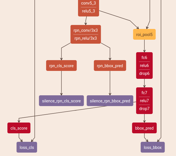
Fast R-CNN train:
- vgg提取特征,得到conv5_3, relu5_3
- roi_pool5: 使用原图roi进行ROIPooing,得到pool5
- pool5进入vgg后两层fc6,fc7
- 两个全连接层
- cls_score,获取21(20个种类+1个背景)种分类概率
- bbox_pred,获取84个点(21 × 4个坐标点)
- 分别计算loss(loss_cls(SoftmaxWithLoss), loss_bbox(SmoothL1Loss))
RoIDataLayer:
RoIDataLayer在RPN训练中返回data,im_info,gt_boxes。
- data,含有所有resize后图片array的blob
- rois=(range(num_rois), x1, y1, x2, y2), 表示原图中roi的数量,4个坐标点
- labels=21个对应的分类标签
- bbox_targets
- bbox_inside_weights
- bbox_outside_weights
这部分具体细节以后补充
ROIPooing
layer {
  name: "roi_pool5"
  type: "ROIPooling"
  bottom: "conv5_3"
  bottom: "rois"
  top: "pool5"
  roi_pooling_param {
    pooled_w: 7
    pooled_h: 7
    spatial_scale: 0.0625 # 1/16
  }
}
输出pool5,shape=(rois个数,conv5的channel个数, pooled_h, pooled_w)
template <typename Dtype>
void ROIPoolingLayer<Dtype>::Reshape(const vector<Blob<Dtype>*>& bottom,
      const vector<Blob<Dtype>*>& top) {
  channels_ = bottom[0]->channels();
  height_ = bottom[0]->height();
  width_ = bottom[0]->width();
  top[0]->Reshape(bottom[1]->num(), channels_, pooled_height_,
      pooled_width_);
  max_idx_.Reshape(bottom[1]->num(), channels_, pooled_height_,
      pooled_width_);
}
Forward 源码 首先计算原图rois映射到feature map的坐标,即原始坐标 x spacial_scale(大小为所有stride的乘积分之一),然后针对pool后每个像素点进行计算,即pool后每个像素点都代表原先的一块区域,这个区域大小为bin_h= roi_height / pooled_ height, bin_w=roi_width / pooled_width。每个像素点的值就是该feature map的区域中最大值,并记录最大值所在的位置。
template <typename Dtype>
void ROIPoolingLayer<Dtype>::Forward_cpu(const vector<Blob<Dtype>*>& bottom,
      const vector<Blob<Dtype>*>& top) {
  const Dtype* bottom_data = bottom[0]->cpu_data(); // conv5_3 feature map
  const Dtype* bottom_rois = bottom[1]->cpu_data(); // 原图roi位置信息
  // Number of ROIs
  int num_rois = bottom[1]->num();
  int batch_size = bottom[0]->num(); // conv5_3 feature map的batch size
  int top_count = top[0]->count();
  Dtype* top_data = top[0]->mutable_cpu_data();
  caffe_set(top_count, Dtype(-FLT_MAX), top_data);
  int* argmax_data = max_idx_.mutable_cpu_data();
  caffe_set(top_count, -1, argmax_data);

  // For each ROI R = [batch_index x1 y1 x2 y2]: max pool over R
  for (int n = 0; n < num_rois; ++n) {
    int roi_batch_ind = bottom_rois[0];
    // 记录原图roi对应在conv5_3 feature map的4个坐标点
    int roi_start_w = round(bottom_rois[1] * spatial_scale_);
    int roi_start_h = round(bottom_rois[2] * spatial_scale_);
    int roi_end_w = round(bottom_rois[3] * spatial_scale_);
    int roi_end_h = round(bottom_rois[4] * spatial_scale_);
    CHECK_GE(roi_batch_ind, 0);
    CHECK_LT(roi_batch_ind, batch_size);

    int roi_height = max(roi_end_h - roi_start_h + 1, 1);
    int roi_width = max(roi_end_w - roi_start_w + 1, 1);
    // 计算一个pool后的像素点对应roi feature map多少个像素点
    const Dtype bin_size_h = static_cast<Dtype>(roi_height)
                             / static_cast<Dtype>(pooled_height_);
    const Dtype bin_size_w = static_cast<Dtype>(roi_width)
                             / static_cast<Dtype>(pooled_width_);

    const Dtype* batch_data = bottom_data + bottom[0]->offset(roi_batch_ind);

    for (int c = 0; c < channels_; ++c) {
      for (int ph = 0; ph < pooled_height_; ++ph) {
        for (int pw = 0; pw < pooled_width_; ++pw) {
          // Compute pooling region for this output unit:
          //  start (included) = floor(ph * roi_height / pooled_height_)
          //  end (excluded) = ceil((ph + 1) * roi_height / pooled_height_)
          int hstart = static_cast<int>(floor(static_cast<Dtype>(ph)
                                              * bin_size_h));
          int wstart = static_cast<int>(floor(static_cast<Dtype>(pw)
                                              * bin_size_w));
          int hend = static_cast<int>(ceil(static_cast<Dtype>(ph + 1)
                                           * bin_size_h));
          int wend = static_cast<int>(ceil(static_cast<Dtype>(pw + 1)
                                           * bin_size_w));
          // height_是conv5_3 height
          hstart = min(max(hstart + roi_start_h, 0), height_);
          hend = min(max(hend + roi_start_h, 0),
          );
          // width_是conv5_3 width
          wstart = min(max(wstart + roi_start_w, 0), width_);
          wend = min(max(wend + roi_start_w, 0), width_);

          bool is_empty = (hend <= hstart) || (wend <= wstart);

          const int pool_index = ph * pooled_width_ + pw;
          if (is_empty) {
            top_data[pool_index] = 0;
            argmax_data[pool_index] = -1;
          }
          // 一个pool像素点的值等于对应conv5_3整个bin_size里最大的值,并且记录该最大值的位置返回
          for (int h = hstart; h < hend; ++h) {
            for (int w = wstart; w < wend; ++w) {
              const int index = h * width_ + w;
              if (batch_data[index] > top_data[pool_index]) {
                top_data[pool_index] = batch_data[index];
                argmax_data[pool_index] = index;
              }
            }
          }
        }
      }
      // Increment all data pointers by one channel
      batch_data += bottom[0]->offset(0, 1);
      top_data += top[0]->offset(0, 1);
      argmax_data += max_idx_.offset(0, 1);
    }
    // Increment ROI data pointer
    bottom_rois += bottom[1]->offset(1);
  }
}
得到了pool5后,接着是就是fc6,这一层InnerProduct先把pool5的输出转换成(roi的个数,channel x width x height),然后每个roi进行InnerProduct计算。
补充几个小的点:
- anchor 生成:
- anchors包括,三个面积尺寸(128^2,256^2,512^2)在各自面积尺寸下,取三种不同的长宽比例(1:1,1:2,2:1)的组合,一共是9个anchor。这里的anchor是指的对应原图的大小的,而总个数是最后一层feature map大小 x 9,14 x 14 x 9,示意图如下:
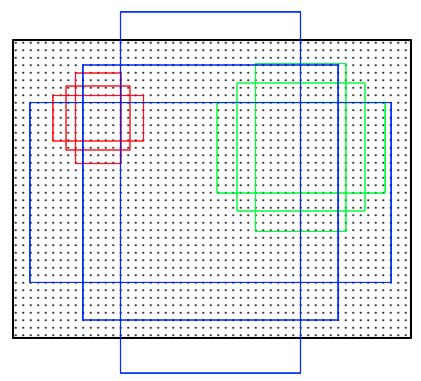
 # 9个anchor的具体坐标点如下
 #array([[ -83.,  -39.,  100.,   56.],
 #       [-175.,  -87.,  192.,  104.],
 #       [-359., -183.,  376.,  200.],
 #       [ -55.,  -55.,   72.,   72.],
 #       [-119., -119.,  136.,  136.],
 #       [-247., -247.,  264.,  264.],
 #       [ -35.,  -79.,   52.,   96.],
 #       [ -79., -167.,   96.,  184.],
 #       [-167., -343.,  184.,  360.]])
- anchors包括,三个面积尺寸(128^2,256^2,512^2)在各自面积尺寸下,取三种不同的长宽比例(1:1,1:2,2:1)的组合,一共是9个anchor。这里的anchor是指的对应原图的大小的,而总个数是最后一层feature map大小 x 9,14 x 14 x 9,示意图如下:
- 为什么vgg16最后一层缩小1/16?(feat_stride为什么是16)
- vgg16中所有的卷积层都是kenel大小(卷积核大小)为3x3,pad大小为1,stride为1的卷积层。用公式W‘ = (W − F + 2P )/S + 1(W代表未经过卷积的feature map大小,F代表卷积核的大小,P代表pad大小,S代表stride大小)计算可以发现,feature map的大小经过卷积后保持不变。vgg16中的卷积层分为5个阶段,每个阶段后都接一个kenel大小为2x2,stride大小为2x2的max pooling,经过一个max pooling后feature map的大小就缩小1/2,经过5次后就缩小1/32。fast rcnn中使用的vgg16只使用第5个max pooling之前的所有层,所以图像大小只缩小1/16。
- rpn为什么使用卷积(3 x 3),(1 x 1)卷积?
- 论文里面写的使用n x n 的sliding windows来映射最后一层feature map对应的特征,实际操作是一个3 x 3 convolution。相当于为RPN网络单独学习提取特征,使得后面两个1 x 1卷积可以学习到对应的信息。这里的1 x 1卷积主要是为了把channel转变为对应的2 x 9, 4 x 9,这样,针对feature map上面每一个点对应的每一个具体的anchor都能有自己的参数,尤其是box regression,可以更加准确。
- rpn中,超出图片大小的anchor处理
- 训练的时候,忽略超出图片大小的anchor,否则会造成很大的误差,并且很难拟合。测试的时候,生成的anchor如果有超出图片大小的会被裁剪掉。
- 为什么使用Smooth L1 loss
-
对输入 x ,输出 f(x) ,标签 Y :L2 loss = f(x) -Y ^{2} ,其导数为 2(f(x) -Y)f’(x); -
L1 loss = f(x) - Y ,其导数为 f’(x) - 因此L1 loss对噪声(outliers)更鲁棒。
-
- 其他一些可能遇到的问题:
- https://blog.csdn.net/u010402786/article/details/72675831?locationNum=11&fps=1
- 一些可以学习的博客:
- https://blog.csdn.net/u014696921/article/details/60321425
Reference:
https://github.com/rbgirshick/caffe-fast-rcnn https://github.com/rbgirshick/py-faster-rcnn https://blog.csdn.net/wfei101/article/details/77778462 https://blog.csdn.net/xyy19920105/article/details/50420779